
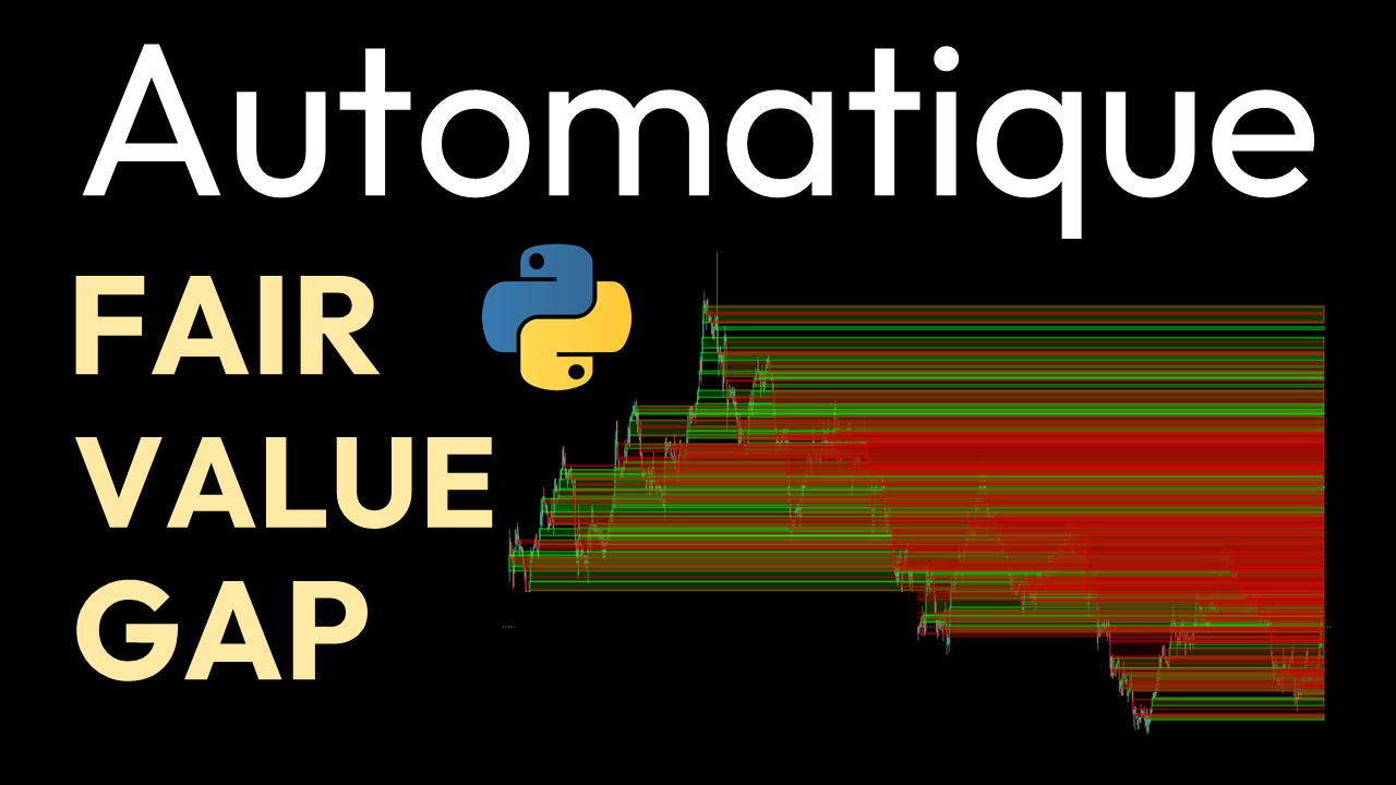
Ce qu’on va faire :
- Télécharger les données EUR/USD
- Détecter les zones FVG bullish et bearish
- Afficher le tout sur un graphique interactif avec couleurs
Charger les données
import yfinance as yf
from lightweight_charts import JupyterChart

TICKER = 'EURUSD=X'
INTERVAL = '3mo'
TIME_FRAME = '1h'

df = yf.download(TICKER, period=INTERVAL, interval=TIME_FRAME, auto_adjust=True)
df = df[['Open','High','Low','Close','Volume']]
df.columns = ['open','high','low','close','volume']
df['time'] = df.index.strftime('%Y-%m-%d %H:%M:%S')
df.reset_index(drop=True, inplace=True)
Dans ce bloc, on récupère les données historiques de l’EUR/USD sur les 3 derniers mois avec des bougies d’une heure grâce à yfinance. Ensuite, on prépare le DataFrame pour lightweight-charts-python en renommant les colonnes et en ajoutant une colonne time au format compatible.
Détecter les FVG
MITIGATION = 0.5

def detect_fvg(df):
    current = df
    previous2 = df.shift(2)

    mitigation_bullish = current['low'] - ((current['low'] - previous2['high'])*MITIGATION)
    mitigation_bearish = current['high'] + ((previous2['low'] - current['high'])*MITIGATION)

    future_highs = df['high'][::-1].cummax()[::-1]
    future_lows  = df['low'][::-1].cummin()[::-1]

    mitigation_not_hit_bullish = (future_lows > mitigation_bullish)
    mitigation_not_hit_bearish = (future_highs < mitigation_bearish)

    fvg_bullish_start = previous2[(previous2['high'] < current['low']) & mitigation_not_hit_bullish]
    fvg_bullish_end   = current[(current['high'].shift(2) < current['low']) & mitigation_not_hit_bullish]

    fvg_bearish_start = previous2[(previous2['low'] > current['high']) & mitigation_not_hit_bearish]
    fvg_bearish_end   = current[(current['low'].shift(2) > current['high']) & mitigation_not_hit_bearish]

    return fvg_bullish_start, fvg_bullish_end, fvg_bearish_start, fvg_bearish_end

bull_start, bull_end, bear_start, bear_end = detect_fvg(df)
Ici, on détecte les Fair Value Gaps (FVG) bullish et bearish. Le MITIGATION = 0.5 sert à filtrer les FVG partiellement comblés. Concrètement si le prix suivant comble 50 % ou plus de la zone du FVG, celle-ci n’est plus considérée comme valide et disparait du graphique.
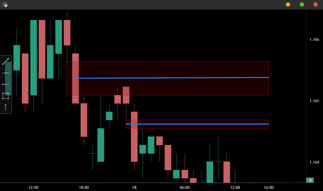
Les FVG avec leur mitigation à 50 % en bleu
Afficher le graphique
df = load_data()
bull_start, bull_end, bear_start, bear_end = detect_fvg(df)
chart = JupyterChart(width=1200, height=600, toolbox=True)
chart.set(df)
draw_fvg(chart, df, bull_start, bull_end, bear_start, bear_end)
chart.load()
Ce code est conçu pour les notebooks (Jupyter, Colab…). L’affichage interactif avec JupyterChart fonctionne directement dans la cellule, mais ne sera pas identique dans un IDE classique. Consulte l’article sur lightweight-charts pour en savoir plus.
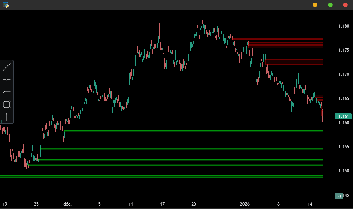
Graphique avec les FVG
Voici le code complet pour afficher le graphique interactif avec les FVG dans un notebook.
import yfinance as yf
from lightweight_charts import JupyterChart

TICKER = 'EURUSD=X'
INTERVAL = '3mo'
TIME_FRAME = '1h'
MITIGATION = 0.5

def load_data():
    df = yf.download(TICKER, period=INTERVAL, interval=TIME_FRAME, auto_adjust=True)
    df = df[['Open','High','Low','Close','Volume']]
    df.columns = ['open','high','low','close','volume']
    df['time'] = df.index.strftime('%Y-%m-%d %H:%M:%S')
    df.reset_index(drop=True, inplace=True)
    return df[['time','open','high','low','close','volume']]

def detect_fvg(df):
    current = df
    previous2 = df.shift(2)
    mitigation_bullish = current['low'] - ((current['low'] - previous2['high'])*MITIGATION)
    mitigation_bearish = current['high'] + ((previous2['low'] - current['high'])*MITIGATION)
    future_highs = df['high'][::-1].cummax()[::-1]
    future_lows  = df['low'][::-1].cummin()[::-1]
    mitigation_not_hit_bullish = (future_lows > mitigation_bullish)
    mitigation_not_hit_bearish = (future_highs < mitigation_bearish)
    fvg_bullish_start = previous2[(previous2['high'] < current['low']) & mitigation_not_hit_bullish]
    fvg_bullish_end   = current[(current['high'].shift(2) < current['low']) & mitigation_not_hit_bullish]
    fvg_bearish_start = previous2[(previous2['low'] > current['high']) & mitigation_not_hit_bearish]
    fvg_bearish_end   = current[(current['low'].shift(2) > current['high']) & mitigation_not_hit_bearish]
    return fvg_bullish_start, fvg_bullish_end, fvg_bearish_start, fvg_bearish_end

def draw_fvg(chart, df, bull_start, bull_end, bear_start, bear_end):
    last_time = df['time'].iloc[-1]
    for (_, start_row), (_, end_row) in zip(bull_start.iterrows(), bull_end.iterrows()):
        chart.box(start_row['time'], start_row['high'], last_time, end_row['low'],
                  color="#00ff1175", fill_color="#00ff1136", width=2)
    for (_, start_row), (_, end_row) in zip(bear_start.iterrows(), bear_end.iterrows()):
        chart.box(start_row['time'], start_row['low'], last_time, end_row['high'],
                  color="#dd00007a", fill_color="#8f00002e", width=2)

df = load_data()
bull_start, bull_end, bear_start, bear_end = detect_fvg(df)
chart = JupyterChart(width=1200, height=600, toolbox=True)
chart.set(df)
draw_fvg(chart, df, bull_start, bull_end, bear_start, bear_end)
chart.load()
N’hésite pas à t’inscrire à la newsletter pour recevoir des insights algorithmiques exclusifs. À bientôt !
ACCÈS MEMBRES
Accès à la newsletter et contenus exclusifs.